| Previous | Table of Contents | Next |
Domain classification
Despite the reduction of the domain pool described above, compression is still very slow compared to other methods such as DCT based algorithms. Another significant speed improvement can be obtained by avoiding domain-range comparisons which have little probability of providing a good match. We assign a class number to each range and each domain, and we compare only members of the same class. To avoid repeated computations, all domains are classified only once at the beginning of the program, by the function classify_domains().
Several methods are possible for classifying ranges and domains. In our sample program, the class is determined in the function find_class() by the ordering of the image brightness in the four quadrants of the range or domain. There are 24 possible orderings, hence 24 classes. For each quadrant we compute the number of brighter quadrants; this is sufficient to uniquely determine the class. Class 0 has quadrants in order of decreasing brightness; class 23 has quadrants in order of increasing brightness.
For simplicity and speed reasons, a range and a domain are compared only with the same orientation. In addition, the contrast factor of affine maps is constrained to be non-negative. After application of such an affine map, the relative ordering of the image brightness in the four quadrants is unchanged. Thus a domain and a range are likely to match well only if they belong to the same class. The validity of this argument can be confirmed in practice by compiling the program with the option -DCOMPLETE_SEARCH. This removes the class restrictions, dramatically increases the compression time, but improves the image quality only very marginally.
Since ranges and domain are compared only with the same orientation, the affine maps are composed in the spatial dimensions of just a scaling by 0.5 and a translation. There is no rotation or symmetry. Thus we do not have to output in the compressed file 3 bits per affine map indicating the selected orientation.
Image partitioning
The encoder can arbitrarily partition the input image into ranges, as long as the decompressor is able to reconstruct the same partition. For simplicity, our sample program uses only square ranges with sizes that are powers of two. We could have further simplified the algorithm by using only ranges 4 pixels wide, but this would not have taken advantage of flat portions of the image, which can be covered well by larger ranges. On the other hand, using ranges that are all 16 pixels wide or larger would not achieve a good quality for the decoded image. Regions of the image with fine detail generally have to be covered with small ranges.
To obtain a good balance between compression ratio and image quality, the function compress_range() first attempts to find a good match for a range 16 pixels wide. If there is no domain which is close enough to the range, that is, if the RMS distance between the range and any domain is greater than the quality value chosen by the user, then the range is split into 4 ranges, and the process is repeated recursively for each of them. When a range is split, the encoder outputs a single zero bit into the compressed stream, to let the decoder know about the need for a split and thus follow the same partitioning algorithm.
In theory, we could allow range splitting up to ranges that consist of a single pixel. This would ensure a perfect quality for the image if the quality factor is selected as zero. For the affine maps, it would be sufficient to chose a null contrast coefficient, and a brightness offset equal to the original pixel value. This would have the additional advantage that image decoding would converge in a single iteration. Unfortunately, all dreams about compression ratios would be gone, since the original file would be expanded instead of being compressed! Therefore it makes sense to impose a minimum size of 4x4 pixels for each range.
The extreme example given above shows, by the way, that it is always possible to find a Partitioned Iterated Function System for a given image; the real problem is to find a good one, which can encode an image with good quality while still offering decent compression ratios.
Since the original image is generally not a square, the function traverse_image() first encodes the largest square fitting in the image, then the two rectangles respectively on the right and below the square. To simplify the algorithm, the size of the square is constrained to be a power of two. If the square is larger than 16x16 pixels, the square is split recursively. We do not attempt to find good matches for regions larger than 16x16 pixels, since it is generally a waste of time: no domain is close enough.
Finding optimal affine maps
The function find_map() finds the best affine map from a range to a domain. This is done by minimizing the RMS distance between range and mapped domain as a function of the contrast and brightness. Actually, we use the sum of squared errors instead of the RMS value to simplify the algorithm and avoid a square root operation. This error value is:
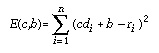
where c is the contrast factor, b the brightness offset, n the number of pixels in the range, di the pixel values in the domain and ri the pixel values in the range. The optimal values of c and b are obtained when the partial derivatives E(c,b) with respect to c and b are both null. The resulting linear equations are easily solved. The values of c and b obtained in this manner are floating point numbers. To ensure a compact encoding of the affine map, these values are quantized and written to the output file as integers using 4 bits for the contrast and 6 bits for the brightness. Using 5 and 7 bits or more would provide a marginally better image quality at the expense of the compression ratio.
The error value E(c,b) is computed using the quantized values of c and b, since the decoder will only know these and not the original floating point values. The error value must depend on the affine map actually selected, not the theoretical best map. There can be a large difference between the optimal contrast and the actual selected contrast since before the quantization, c is restricted to the interval 0.0—1.0. The lower bound is needed because of our simple domain classification mechanism, the upper bound is needed to ensure that the affine map is contractive in the luminance dimension.
| Previous | Table of Contents | Next |